A unified perspective of RLHF

Currently popular RLHF Method

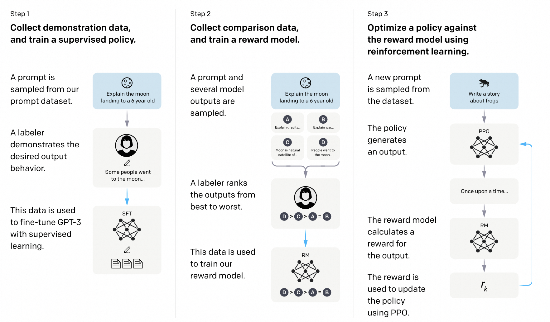
To this day，the post-training diagram for LLMs is still CPT, SFT and RLHF. There are no signs that this diagram will change currently. Focusing on RLHF, I will attempt to provide a comprehensive review, summary and future outlook in the following, in order to clarify its development path and hopefully gain some interesting insights.

Preliminaries

Potential-Based Reward Shaping (PBRS)

Definition

A shaping reward function $F : S \times A \times S \to \mathbb{R}$ is potential-based if there exists $\Phi : S \to \mathbb{R}$ such that:

$$F(s, a, s') = \gamma \Phi(s') - \Phi(s)$$

for all $s \neq s_0, a, s'$.

PBRS cleverly introduces the concept of potential, guiding the agent to search more quickly in the state space without altering the optimal policy of the original problem.

Policy Invariance Under Reward Transformations: Theory and Application to Reward Shaping

Policy Gradient Algorithm

As a reinforcement learning algorithm that directly optimizes the policy itself, policy gradient methods compute a estimator of the gradient and optimize it using the gradient ascent algorithm. Specifically, this estimator is generally:

$$\hat{g} = \hat{\mathbb{E}}_t \left[ \nabla_\theta \log \pi_\theta(a_t \mid s_t) \hat{A}_t \right]$$

where $\pi_\theta$ is the stochastic policy and $\hat{A}_t$ is the estimator of the advantage function at timestep $t$.

So the estimator $\hat{g}$ is actually obtained by differentiating the objective:

$$L^{PG}(\theta) = \hat{\mathbb{E}}_t \left[ \log \pi_\theta (a_t \mid s_t)\hat{A}_t \right].$$

However, directly using $L^{PG}$ as a loss for optimization may lead to excessively large policy updates, potentially pushing the policy away from well-performing regions, and it often performs poorly in practice. Therefore, various methods such as PPO are typically used, as they incorporate mechanisms to control update sizes and ensure more stable and efficient learning.

Generalized Advantage Estimator(GAE)

GAE is a widely applicable advantage estimation method that can effectively reduce the variance of gradient estimation in policy gradient methods. The formula of GAE is:

$$\hat{A}_t^{GAE(\gamma, \lambda)} = \sum_{l=0}^{\infty} (\gamma \lambda)^l \delta_{t+l}^V = \sum_{l=0}^{\infty} (\gamma \lambda)^l (r_{t+l} + \gamma V(s_{t+l+1}) - V(s_{t+l}))$$

High-Dimensional Continuous Control Using Generalized Advantage Estimation

TRPO(Trust Region policy optimization)

TRPO maximizes an objective function while subjecting it to a constraint on the size of the policy update. Specifically:

$$\text{maximize}_{\theta} \, \hat{\mathbb{E}}_t \left[ \frac{\pi_\theta(a_t \mid s_t)}{\pi_{\theta_{\text{old}}}(a_t \mid s_t)} \hat{A}_t \right]$$

subject to $\hat{\mathbb{E}}_t[\text{KL}[\pi_{\theta_{\text{old}}}(\cdot \mid s_t), \pi_\theta(\cdot \mid s_t)]] \le \delta$, where, $\theta_{\text{old}}$ is the policy parameters before the update.

By incorporating a penalty term in the objective function to control the size of policy updates, the problem becomes an unconstrained optimization problem:

$$\text{maximize}_{\theta} \hat{\mathbb{E}}_t \left[ \frac{\pi_\theta(a_t \mid s_t)}{\pi_{\theta_{\text{old}}}(a_t \mid s_t)} \hat{A}_t - \beta \text{KL}[\pi_{\theta_{\text{old}}}(\cdot \mid s_t), \pi_\theta(\cdot \mid s_t)] \right]$$

where $\beta$ is the coefficient. However, experiments show that using a fixed $\beta$ and optimizing the upper objective with SGD is insufficient, which leads to the development of PPO.

Methods

PPO(Proximal Policy Optimization)

PPO - CLIP

We define that $r_t(\theta) = \frac{\pi_{\theta}(a_t|s_t)}{\pi_{\theta_{old}}(a_t|s_t)}$, then the main objective proposed by PPO is:

$$L^{\text{CLIP}}(\theta) = \hat{\mathbb{E}}_t \left[ \min \left( r_t(\theta) \hat{A}_t, \text{clip}(r_t(\theta), 1 - \epsilon, 1 + \epsilon) \hat{A}_t \right) \right]$$

where $\epsilon$ is the hyperparameter. This formulation ensures that $r_t(\theta)$ remains within a certain range, preventing $\pi_{\theta}(a_t|s_t)$ from deviating too much from $\pi_{\theta_{old}}(a_t|s_t)$.

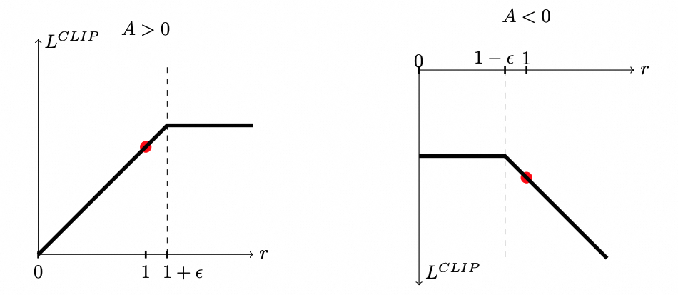
The choice between $1 + \epsilon$ and $1 - \epsilon$ depends on the sign of the advantage function $\hat{A}_t$.

When $\hat{A}_t > 0$ (i.e., the current action is better than the baseline):

Increasing $r_t(\theta)$ (i.e., the new policy is more inclined to choose this action) will enhance the objective function because it amplifies the positive advantage. However, to prevent excessively large policy updates that could destabilize training, if $r_t(\theta) > 1 + \epsilon$, the clipped term $(1 + \epsilon) \hat{A}_t$ will be smaller than the unclipped term $r_t(\theta) \hat{A}_t$. Since the objective function takes the minimum of the two, in this case, the clipped term $(1 + \epsilon) \hat{A}_t$ will be selected, thereby ignoring further increases in $r_t(\theta)$ that would otherwise beneficially change the objective.

When $\hat{A}_t < 0$ (i.e., the current action is worse than the baseline):

Decreasing $r_t(\theta)$ (i.e., the new policy is less inclined to choose this action) will enhance the objective function because it reduces the impact of the negative advantage. If $r_t(\theta) < 1 - \epsilon$, the clipped term $(1 - \epsilon) \hat{A}_t$ will be smaller than the unclipped term $r_t(\theta) \hat{A}_t$ (since $\hat{A}_t$ is negative). In this case, the clipped term $(1 - \epsilon) \hat{A}_t$ will be selected, thereby preserving $r_t(\theta)$ from decreasing too much.

In fact, the role of $L^{\text{CLIP}}$ is to constrain the updates of $r_t(\theta)$ within a certain range.

PPO - Penalty

PPO-penalty employs several epochs of minibatch SGD to optimize the KL-penalized objective given by:

$$L^{KL PEN}(\theta) = \hat{\mathbb{E}}_t \left[ \frac{\pi_\theta(a_t \mid s_t)}{\pi_{\theta_{\text{old}}}(a_t \mid s_t)} \hat{A}_t - \beta \text{KL}[\pi_{\theta_{\text{old}}}(\cdot \mid s_t), \pi_\theta(\cdot \mid s_t)] \right]$$

then computes $d = \hat{\mathbb{E}}_t[\text{KL}[\pi_{\theta_{\text{old}}}(\cdot \mid s_t),\pi_\theta(\cdot \mid s_t)]]$

• If $d < d_{\text{targ}}/1.5$, $\beta \leftarrow \beta/2$
• If $d > d_{\text{targ}} \times 1.5$, $\beta \leftarrow \beta \times 2$

where $d_{targ}$ is a pre-set hyperparameter used to limit the difference between the current policy and the policy from the previous iteration. The updated $\beta$ is used for the next policy update.

Apparently, PPO-penalty imposes less strict constraints on the magnitude of policy updates compared to PPO-clip, and its performance in experiments is also inferior to the latter according to the PPO paper.

PPO’s Advantage Estimator

PPO adopts a truncated generalized advantage estimator(GAE), when $\lambda = 1$:

$$\hat{A}_t = \delta_t + (\gamma \lambda) \delta_{t+1} + \cdots + (\gamma \lambda)^{T-t+1} \delta_{T-1},$$

where $\delta_t = r_t + \gamma V(s_{t+1}) - V(s_t)$. In RLHF, $r_t$ is provided by the reward model, generally using the following formula:

$$r(s_t, \mathbf{a}_t) = \begin{cases} \beta \log \pi_{\text{ref}}(\mathbf{a}_t|s_t), & \text{if } s_{t+1} \text{ is not terminal} \\ r(\mathbf{x}, \mathbf{y}) + \beta \log \pi_{\text{ref}}(\mathbf{a}_t|s_t), & \text{if } s_{t+1} = \mathbf{y} \text{ is terminal} \end{cases}$$

$V(s_t)$ is given by the critic model, which fits the expected return by calculating an MSE loss with the actual return $R_t=r_t + r_{t+1} + ... + r_T$.

DPO

ORPO

KTO

IPO

SimPO

High-Dimensional Continuous Control Using Generalized Advantage Estimation

Proximal Policy Optimization Algorithms

Direct Preference Optimization: Your Language Model is Secretly a Reward Model

https://lilianweng.github.io/posts/2018-04-08-policy-gradient/

关于LLM+RL(HF)的片面脉络梳理